UPDATE: The post below has been updated to reflect the Democratic flip of CA-21 and the results of the Mississippi special election. It is now up-to-date as of November 29th.
Introduction
The following document presents preliminary analysis of the performance of the Øptimus House and Senate models, as well as how they compare to other forecasting models and ratings. Overall, both the House and Senate models performed great and stacked up very well against other forecasts.
Included in our preliminary analysis are the 434 House races and 34 Senate races that have been called by most outlets as of November 29th. If any unexpected surprises pop up, the numbers presented below are subject to (minimal) change.
Our final House prediction had Democrats at a 95.9% chance of taking control of the chamber. The mean prediction was 233 Democratic seats to 202 GOP seats, and the 90% confidence interval spanned from 218 Democratic seats to 248. Control of the House was called early in the night by most outlets and was only in doubt at all due to jitters about early Senate results and sensitive live forecasts that were prominent on Election night. The exact number of seats won by each party is not yet final, but based on the current trajectory, it looks like Democrats will end up with 235 seats, and Republicans with 200.
On the Senate side, our final prediction gave Republicans a 91.9% chance of keeping control of the chamber. The mean seat prediction was 52 GOP seats to 48 Democratic seats, with a 90% confidence interval spanning from 49 GOP seats to 55 GOP seats. Our GOP chance of keeping the majority peaked above 89% at three different points: in mid-August, in mid-October, and right before the election. As with the House race, the chamber control prediction we expected was called very early on in the night, with Democrats (somewhat surprisingly) struggling in Indiana and Florida. The actual number of GOP seats appears to have settled at 53.
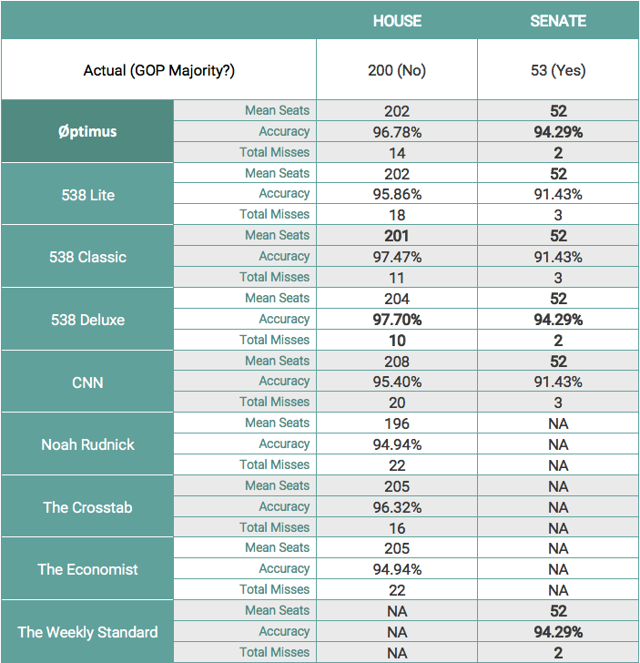
The following table shows several metrics relevant in comparing our model to other public House and Senate models. For each model, the mean seats, accuracy, and total misses are presented. Our House model will likely be within 1 seat of the actual seat total. 538’s Deluxe model led the way on accuracy at 97.9%, with the Øptimus model right behind at 97.0%. In the Senate all 6 models predicted 52 GOP seats, though only 3 correctly assessed Missouri – Øptimus, 538 Deluxe, and The Weekly Standard. The Øptimus model missed the same two races as those two outlets (Florida and Indiana) though by smaller margins (we had Indiana at 41% and Florida at 32%).

The remaining sections go more in-depth on individual predictions. The first two demonstrate metrics for our model itself, as well as the sub-models used in the creation of our ensembles. The next two sections compare our models to those of other public forecasters – both quantitative and qualitative.
Model Performance
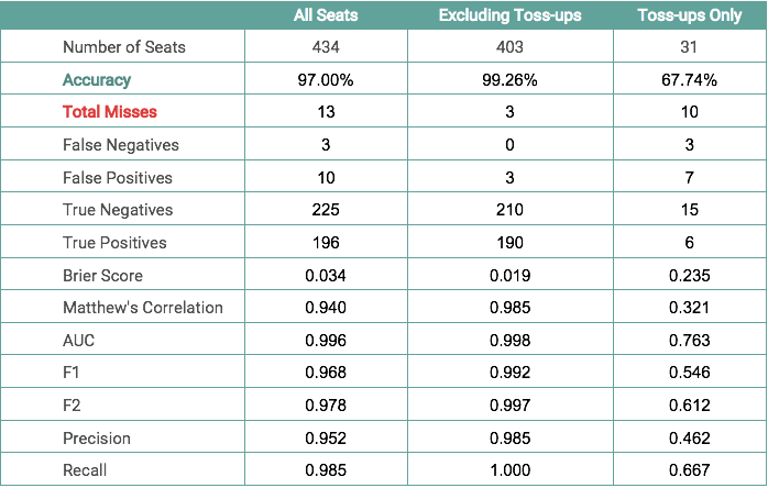
The following table contains the performance scores for the Øptimus House model. As of November 26th, for the 434 races called, the Øptimus House model called 421/435 races correctly, meaning the model has an accuracy of 96.78%. Among the 31 toss-ups, the model predicted 21/31 toss-up races correctly, meaning it has 67.74% accuracy among these races. Excluding the toss-ups, the House model is 99.01% accurate, meaning it predicted 400 out of 404 non-toss-up races correctly.
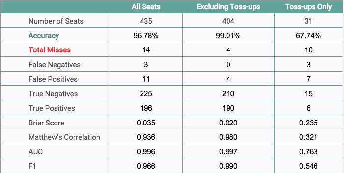
The table below contains the performance scores for the Øptimus Senate model. As of November 29th, for the 35 races, the Øptimus Senate model has an accuracy of 94.29%, meaning the models predicted 33 out of 35 races correctly. Among the 4 toss-ups called, the model correctly predicted 3 out of 4 races. Out of the 31 non-toss-ups, the only race missed by the Senate model is the Florida Senate seat.
Performance Analysis Of Individual Models Within The Ensemble
Most election forecasting models utilize either a Bayesian approach or classical logistic regression to predict the outcome of an election. Our modeling process utilizes an ensemble technique, incorporating various algorithms and variable subsets, including Bayesian logistic regression Random Forest, XGBoost and Elastic Net to forecast an election. Including a variety of algorithms and variable subsets in our ensemble reduces error in two ways. First, ensembles have proven to be more accurate on average than their constituent models alone. Second, they are less prone to making substantial errors (if they miss, they miss by smaller margins on average) (Montgomery et al. 2011). Individual models produce good results but will give slightly different estimates for each race. On the whole, we have found them to be comparable based on accuracy and f1 score, but they produce better estimates when averaged together. In our testing, the ensemble predictions produce fewer misses in 2014 and 2016 than any single model alone.
In the House model, we combine two separate ensemble models to leverage both party-oriented variables as well as incumbency-based variables, to which we add any recent polling information. In the Senate, a single party-oriented ensemble model is sufficient to produce accurate results and is later combined with polls to make a final prediction.
In both the House and Senate, our ensemble of individual models and polls performs better than individual models based on accuracy, Brier score, MCC, F1 and F2 scores. This implies that an ensemble of individual models combined with polls performs better than individual models with respect to calibration as well as classification. We expected this to be the case based on back-tests of 2014 and 2016 performed in advance.
In the House and Senate models, the Bayesian model outperforms every other individual model in terms of accuracy. Bayesian statistics, in a simplified manner, consists of utilizing observed data to update our degree of belief in an event occurring. For our purposes, the outcome of a GOP win in a particular race is modeled as a Bernoulli random variable with success probability θ. The success probability θ is modeled as a function of the features in the dataset using logistic regression. Parameters of the logistic regression are drawn from non-informative prior distributions, such as the student-t distribution which is similar to the normal distribution but has higher chance of sampling unlikely events. We use JAGS, a program for analysis of Bayesian models using Markov Chain Monte Carlo (MCMC) simulations, to obtain the posterior distributions of the parameters used in the logistic regression. Posterior distributions of the parameters can be thought of as informed distributions, obtained by updating prior distributions using the data. Using the posterior distributions of these parameters, we derive the probability distribution of a GOP victory in each district for the 2018 midterm elections.
The following table shows the accuracy and total number of incorrect predictions made by every individual model included in the ensemble, as well as by the final ensemble of individual models and polls.
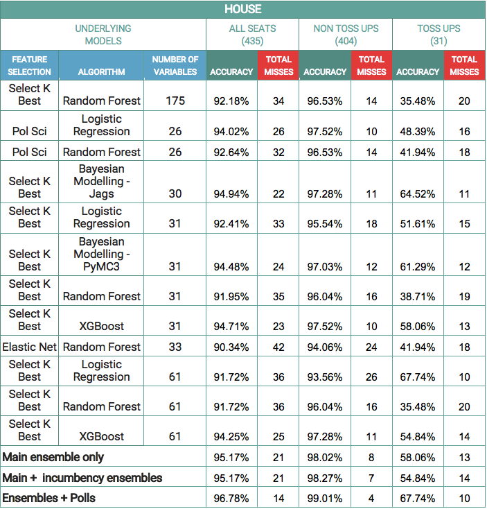
The following table shows the accuracy and total number of incorrect predictions made by every individual model included in the ensemble, as well as by the final ensemble of individual models and polls.
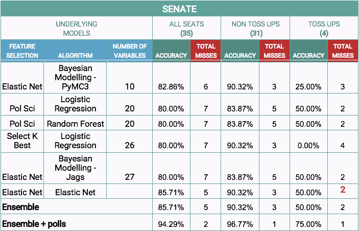
A linear combination of the chances of GOP victory based on ensemble of individual models and polls gives the best performing model. We have observed this in our out-of-sample back-tests (2016, 2014, 2010, and 2006) as well. Creating an ensemble of individual models helps to minimize the systematic bias in each of the models. In this way, weaknesses of individual models can be compensated by combining them together.
There are many factors that may or may not be captured by historical data, (e.g. scandals, or any non-historical trends). Our models heavily depend on financial spending by a candidate, and hence it can produce over-confident predictions in favor of candidate that outspends his/her opponent. We compensate for such biases using probabilities calculated using recent polls. Therefore, we combine probabilities calculated using historical data with polling data, to produce our final prediction, thereby reducing systematic bias in our models using ensemble technique and accounting for non-historical information by using polls.
Comparison To Other Quantitive Models
Now we compare how our 2018 midterm forecast held up against other quantitative models. On the Senate side, we’ll compare our model against 5 probabilistic forecasts from 3 of the most reputable outlets covering the election: one model each from CNN and The Weekly Standard and 3 models from FiveThirtyEight (Lite, Classic and Deluxe).
Each of the forecasters correctly predicted that Republicans would maintain control of the Senate with various levels of certainty. Among forecasters that provided a specific probability of a Republican majority, Øptimus was the most certain (91.9%) that the GOP would keep the Senate.
The individual Senate seat forecasts fall into two basic categories: those that correctly picked Missouri and those that did not. It was the only race upon which the forecasters disagreed, with CNN, FiveThirtyEight Lite and FiveThirtyEight Classic incorrectly picking Claire McCaskill (D), and Øptimus, The Weekly Standard and FiveThirtyEight Deluxe correctly picking Joshua Hawley (R), who won by 6 percentage points. All of the models missed on Indiana and Florida Senate seats.
The following table compares model evaluation metrics among the 6 Senate forecasts.
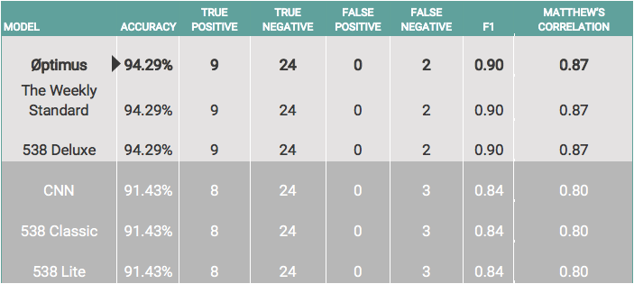
One thing worth noting is that none of the forecasts produced any false positives; in other words, if any of the forecasts gave the Republican the edge, the Republican won 100% of the time. In that regard, Republicans overperformed on the Senate side relative to their projected odds, winning two races (Indiana and Florida) in which none of the forecasters had them favored.
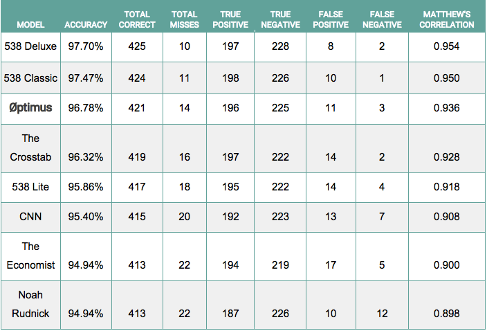
Moving onto the House forecasts, a few more forecasters enter the fray. We compare one model each from The Crosstab, CNN, The Economist, and Noah Rudnick, and 3 models again from FiveThirtyEight. Each of the forecasters correctly predicted that Democrats would gain control of the House with varying degrees of certainty. Among forecasters that provided a specific probability of a Democratic majority, Øptimus was the most certain (95.9%) that the Democrats would successfully flip control of the House.
The Øptimus House model performed exceptionally well when compared with the other forecasts in terms of accuracy, trailing only FiveThirtyEight’s Deluxe and Classic forecasts with 1 race still to be decided.
Comparison To Qualitative Ratings
While our model is quantitative, we also assign our predictions into bins that resemble those made by qualitative raters like Cook, Sabato’s Crystal Ball, and Inside Elections. Our ratings correspond to categories as follows:
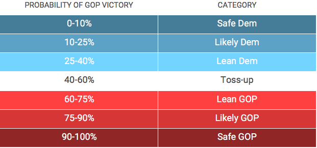
With these categories, our model becomes comparable to Cook Political, Larry Sabato’s Crystal Ball, and Inside Elections ratings. Since these are qualitative, judging them becomes more subjective. In general, you would want ratings that are not “wrong” (e.g., Lean D are not won by Republicans often and vice versa), but also those that do make predictions about where races sit (you can be “right” on all competitive races by labeling them all toss-ups, but this isn’t informative).
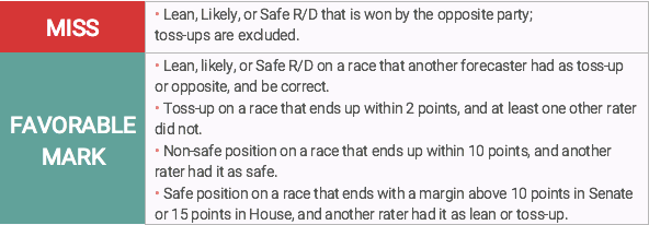
With these in mind, we created a positive/negative rubric for judging how well a given set of ratings did. First, we count “misses,” which are when a race receives a rating besides toss-up, and the opposite party wins the race. Second, we use a metric we’ll call “favorable marks,” which are earned when a rating ends up being an accurate representation of where a race stands relative to other raters. The idea is to reward a set of ratings for correctly pinpointing the state of a race while other ratings (or put a different way, the “conventional wisdom”) had it at least a bit off.
There are four scenarios that earn favorable marks: races in which you take a position on a race, get it right, and one of the other organizations had it as a toss-up; races in which you rate the race as a toss-up, and the final margin is within 2 percentage points; races that are rated not safe D or safe R, and the final margin is less than 10 percentage points, and at least one other organization had it as safe; and races that are rated safe D or safe R, the final margin is more than 10 percentage points in the Senate or 15 points in the House, and another organization had it as lean or toss-up. The chart below summarizes misses and favorable marks.
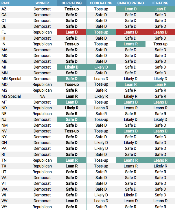
On the Senate side, the following table summarizes the differences in each rating. Our ratings earned 5 favorable marks, while Cook earned 2, Sabato’s Crystal Ball earned 6, and Inside Elections earned 5. Our ratings, Crystal Ball, and Inside Elections each have one miss (Florida), while Cook had none.
Cook was extremely risk-averse this year. They had 9 toss-up races, while we had 4, Sabato had 0, and Inside Elections had 1. This explains why Sabato and Inside Elections did well (they made actual predictions that were correct on all but Florida), while Cook struggled by our metric. They included races spanning from New Jersey, where Menendez (D) won by 11 percent, to Tennessee, where Blackburn (R) won by 11 percent. Both of those races were in reality fairly lopsided.
Our ratings were more representative of the state of races than Cook, though Crystal Ball and Inside Elections both nailed Missouri, and Crystal Ball correctly rated Indiana (we had both as toss-up).
The table below showcases the House version. The Øptimus and Cook ratings lead the way with only 4 total misses, with Inside Elections at 6 misses and Sabato’s Crystal Ball assigned a lean to each race and missed on 14. Because they did so, Crystal Ball also had the most favorable marks, at 30. Inside Elections had 23, Øptimus had 21, and Cook was once again very risk-averse and therefore had 19.

Recap
Overall, the Øptimus House and Senate models performed exceptionally well. On the surface, they correctly predicted which party would control each chamber, the mean of each model came within 1-2 seats of the actual seat outcome and had high accuracy in doing so. Compared to other models, the Øptimus models performed at the same level as the most reputable public models and outdid most of them. Combined with the out-of-sample back-tests performed on previous years, this performance indicates that our approach to election modeling predicts legislative election outcomes with a high level of accuracy, both at the individual seat level and aggregate level. We’re looking forward to our 2020 model and looking into other applications for our technique.